The GêBR Project kindly thanks the support of:
- Brazilian oil company, Petrobras.
- Brazilian Geophysical Society (SBGf).
- National Institute for Petroleum Geophysics (INCTP-GP).
- Brazilian universities and research centers.
Table of Contents
List of Figures
- 2.1. Add header flows
- 2.2. Communication layout between GêBR players
- 2.3. Another node assumes the maestro position whenever necessary
- 3.1. Projects and Lines tab
- 3.2. Dialog for lines from domain with disconnected domain
- 3.3. Built-in commentary editor
- 3.4. View Report
- 3.5. Report menu
- 4.1. Flows tab
- 4.2. Filtering the menus list
- 4.3. Input file setting
- 4.4. Autocomplete of paths
- 4.5. Run and Setup
- 5.1. Dictionary of variables
- 5.2. Loop program
- 5.3. Loop parameters
- 5.4. Usage of iter variable
- 5.5. Snapshots on GêBR
- 5.6. Dialog of Reverting modified flow
- 6.1. Jobs tab
- 6.2. Jobs tab left panel
- 6.3. Details of job execution
- 6.4. Jobs outputs
- 7.1. Global GêBR preferences dialog box
- 7.2. Maestro / Nodes configuration dialog box
- 8.1. GêBR public-key authentication
- 8.2. Remote browsing of files
- 8.3. Indication of MPI availability
- 8.4. MPI settings
List of Tables
- 5.1. Available functions
List of Examples
- 4.1. Parallel execution
- 5.1. Using the dictionary
- 5.2. Using snapshots
- 7.1. Using the groups
GêBR is a simple graphical interface which facilitates geophysical data processing. GêBR is not a package for processing. Instead it is designed to integrate a large variety of free processing packages, such as Seismic Un*x and Madagascar.
GêBR manages seismic-data processing projects, dealing with multiple 2D lines, each one with its own set of processing flows. Through GêBR, it is possible to assemble and execute such processing flows and track the outputs of the data processing. Everything in a simple and friendly way.
Being a free software, anyone can use and customize GêBR for free, according to the terms of the GNU Public License. That makes this software very attractive for teaching and academic research.
The GêBR Project was initially proposed to develop and promote the GêBR interface. During 2007–2008, the core team of developers had offered several courses on seismic processing with GêBR, at the most active research centers in Geophysics in Brazil. Around 200 students and professionals had direct contact with the project on that period. In that process the GêBR observed a demand for integration efforts among Brazilian geophysical community. That motivated a redefinition for the project’s goals.
The main objective of GêBR is to stimulate the integration of the Brazilian Geophysical Community by providing an interface to geophysical data processing that could be used not only for teaching purposes but also as a research dissemination vehicle.
For more information, visit the project's official site: http://www.gebrproject.com.
-
Version 0.20.0 (current)
This release of GêBR brings a lot of new exciting features to ease the handling and the management of flows and programs, including:
- Joining of Flow Editor and Flow Browse tabs navigation: now through Flows tab is possible control all actions about flows and programs, thus the activities at GêBR are much more centralized, fast and easy (see Chapter 4, The Flows tab: basic aspects).
- Flows tab powered: the work on GêBR is wonderfully fast, because now it's possible to see in the same tab a summary information of the flow, edit programs and their parameters and also to see the output of the flow's execution. (see Chapter 4, The Flows tab: basic aspects).
- New Toolbar: the new toolbar makes the GêBR interface much more clean. Just the frequently used actions are on the toolbar, the other actions are placed in More menu (see Chapter 3, The Projects and Lines tab and see Chapter 4, The Flows tab: basic aspects).
- Quick access to Menus list: the new toolbar brings a new way of to access the menu list. Through the menu list icon it's possible to see all the menus and add them to the flows in few clicks (see Section 4.1, “The menus list”).
- Execution modes: now there are two options of execution, it's possible run the flows directly or choose and save the preferences of execution and then run the flows. So, it's just necessary changing the preferences once or when it's desired run a flow in a different way from the standard mode (see Section 4.7, “Executing flows”).
- Snapshots: this feature gives much more freedom to the flows, all the important status of flows can be saved and reverted anytime, thus it's possible modify loosely the flows and their programs (see Section 5.4, “Snapshot of a flow”).
- Search on documentation: never more fell lost among the documentation and reports. Starting this release of GêBR it's possible to search terms in the reports of projects, lines and flows and also in the flow summary (see Chapter 4, The Flows tab: basic aspects).
-
Version 0.18.0 (May 24th 2012)
- Prior to this version, lines could have some directories, known as line's paths. Shortcuts to those directories were available in each file browse dialog. From this version, to each line it is associated a standard hierarchy of directories (see definition in Section 3.3, “Important folders of a line” and example of usage in Section 4.5, “Editing the flow's input and output files”).
- Now it's possible to change the line's maestro (see Section 3.4, “Changing the domain of a line”).
- GêBR correctly displays remote folder (see Section 8.2, “Accessing remote files”).
-
Version 0.16.0 (January 30th 2012)
- The concept of Maestro is born, allowing to execute jobs in multiples machines. (see Section 7.3, “Maestro/Nodes configuration” and Section 8.3, “Parallelized processing”).
- Now it is possible to control the number of cores used by the jobs of GêBR and change the priority of execution of a job (see Section 8.3, “Parallelized processing” and Section 8.4, “Priority of execution”).
- Renewed interface: new functionalities and improved usability.
-
Version 0.14.0 (October 3rd 2011):
- The variables dictionary and the program parameters accept arithmetic expressions (see section Section 5.2, “Using variables”).
- Repetitive processes can be automatized by the use of loops (see section Section 5.3, “Flows with loops”).
This user guide is for GêBR version 0.20.0. The images in this guide were captured in a Ubuntu 10.04 based system. Therefore, slight differences may be observed in case another operating system is being used. For specific installation instructions for each operating system, see the install guide, in the project's official site.
Director:
-
Ricardo Biloti
<biloti@gebrproject.com>
Developer manager:
-
Fabrício Matheus Gonçalves
<fmatheus@gebrproject.com>
Developers:
-
Eric Keiji
<keiji.eric@gebrproject.com> -
Ian Liu Rodrigues
<ian.liu@gebrproject.com> -
Igor Henrique Soares Nunes
<igor.snunes@gebrproject.com> -
Jorge Pizzolatto
<jorge.pzt@gebrproject.com> -
Júlia Koury Marques
<juliakm@gebrproject.com> -
Vinícius Oliveira Querência
<querencia@gebrproject.com>
Consultants:
- Bráulio Oliveira
- Eduardo Filpo
- Fernando Roxo
- Luis Alberto D'Afonseca
- Rodrigo Portugal
Former members:
- Alexandre Baaklini
- Davi Clemente
- Fábio Azevedo
- Gabriel Sobral
- Giuliano Roberto Pinheiros
- Priscila Moraes
- Renan Giarola
- Rodrigo Morelatto
Thank you for using GêBR!
Table of Contents
GêBR is primarily conceived to process 2D seismic data lines. Data from 2D acquisition lines related somehow are usually grouped in one seismic-data processing project. The processing of a specific data is carried out by a bunch of processing flows. Each processing flow is a chain of programs, which sequentially operate on an input data to produce an output data from it. For example, processing flows can be assembled to accomplish tasks like Spike Deconvolution, Noise Atenuation, NMO correction, and so on.
In GêBR, a seismic-data processing project is referenced as a project only. Each project can hold many seismic data, each one referenced as a line. Each line has its own set of processing flows or just flows for short.
In summary, GêBR has three levels organization, from top to bottom:
-
Project: It is a set of lines. A project has only a few basic information and is used to cluster lines related somehow.
-
Line: It is a set of flows. During the setup of the line, some important choices have to be made, mainly concerning the organization of the processing products (intermediate data, figures, tables, etc) produced during the processing of the seismic data.
-
Flow: It is a sequence of programs, designed to accomplish a specific task, in the course of seismic data processing.
Thus, before creating and executing flows, it's necessary to create at least one project owning one line. Section 3.1, “Creating projects and lines”, and Section 4.2, “Creating flows” explain how this is accomplished.
To assemble a flow, the user has not only to select programs, but also configure them properly, through their parameters. Once the flow is configured, it is ready to actually be executed.
A flow is a sequence of programs, as just explained. In GêBR, the user might think that there is a list of available programs to assemble flows. This is partially true only. Indeed, flows are built from menus. But what is a menu?
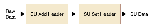
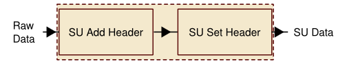
A menu is a representation of a single program or a set of programs. This means that when a menu is added to a flow one or more programs will be inserted into the flow at once. Why is that so? Think about common tasks that are accomplished by a standard sequence of programs. Instead of building a flow by adding programs one by one, the flow could be built from a menu, which packs the whole set of programs. For example, consider the task of adding header to a raw data to come up with a seismic data in Seismic Un*x format. Figure 2.1, “Add header flows” shows two possibilities to assemble the same flow, depending on how the programs SU Add Header and SU Set Header are represented, either as two independent menus or as one menu encapsulating both programs.
Figure 2.1. Add header flows
Note
Even when a menu represents more than one program, at the moment the menu is added to the flow, all programs which comprises it are added independently to the flow. This means that resulting flow will be the same, no matter how the programs have been added, at once or one by one.
After assembling the flow, to complete its set up, the user has to inspect each program of the flow and define its parameters. Programs may depend on many parameters, from a variety of types. GêBR supports parameters of the following types:
- Numeric
- Text
- Booleans
- Files
- List of options
Tip
GêBR supports arithmetic expressions to define numeric parameters, and text concatenation for text parameters. Besides, it is possible to define quantities and operate with them to set up parameters of the programs.
The GêBR set of tools is composed by two main player categories: GêBR (the interface itself) and nodes.
The GêBR interface, sometimes referred as GêBR only, is the graphical interface with whom the user interacts to build flows, execute them, inspect results, etc. Usually, this interface is installed and is running in the machine the user has physical contact with.
The user may have access to many machines, which is an usual scenario for users of a computational laboratory. Through GêBR, it is possible to take advantage of these machines. A machine used to run processing flows is called a processing node, or just node, for short. They may be local, meaning the user is physically using them, or remote, meaning the user has access to them through the network. No matter where the machines are, they are equally treated by GêBR, which means that the user does not have to care about that.
Whenever machines can cooperate to run processing flows, they are grouped into domains. Basically a domain is a set of processing nodes that have access to the same files in disk, and therefore can operate on the same data sets.
GêBR does not talk directly to each node of a domain. Instead, it elects one processing node of the domain to be responsible to receive all requests from the interface and redistribute them to the processing nodes. This special node is called maestro. Any node can assume this function.
Figure 2.2. Communication layout between GêBR players
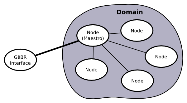
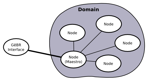
In case the machine acting as the maestro fails or is no longer accessible to the GêBR interface, another processing node assumes this function.
When the user decides to execute a flow, GêBR sends the request to the maestro, giving rise to a job. The maestro acts as a coordinator of the nodes into the domain, collecting information and ranking them according to their capabilities and available resources. Therefore, the maestro can take smart decisions about which machines are best suited to run a job.
The nodes put their computational power at disposal of the maestro. Under maestro's coordination the nodes can even cooperate to conclude processing jobs fasters.
The maestro receives the job submission and dispatches the job to some of the nodes under its control. All the information generated by the job is collected and sent back to GêBR, where they are presented to the user.
This communication process, despite complex, is completely transparent to the user, which can concentrate on processing seismic data, leaving all technical details to GêBR.
The GêBR interface is intentionally simple. It is organized in three tabs:
- Projects and Lines: For creating and manipulating projects and lines;
- Flows: For creating, editing and executing flows;
- Jobs: For inspecting the results.
There are also additional resources in menu bar, on the top of the window:
-
Actions
- Preferences: User preferences;
- Connections Assistant: Step-by-step guided setup of the main connections performed by GêBR;
- Maestro/Nodes: Configuration of maestro, nodes and groups of nodes;
- Quit: Quits GêBR.
-
Help
- Help: This documentation;
- Samples: Examples of seismic processing;
- About: GêBR's version, license and staff information.
Table of Contents
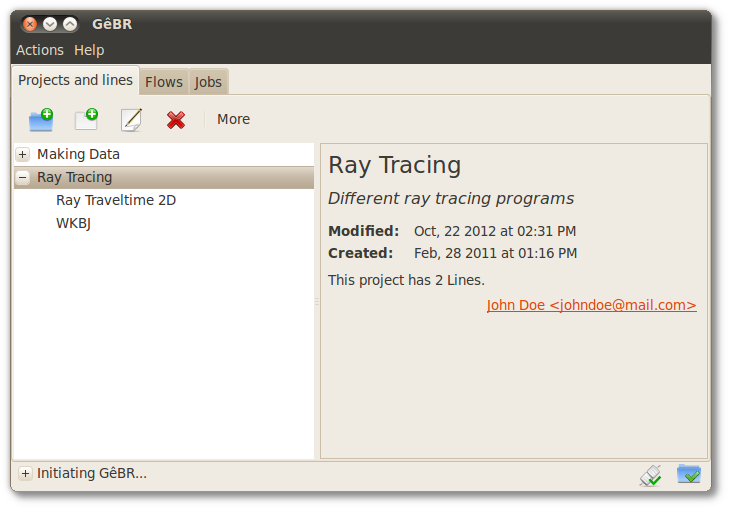
Projects and lines are the organizer entities (see Section 2.1, “Projects, lines and flows”). They are created and managed in the Projects and Lines tab. Lines are grouped in projects, for sake of organization. The information presented in the Flows tab depends on the line selected at the moment.
Figure 3.1. Projects and Lines tab
Tip
Try using a context menu instead of the buttons on the toolbar. To do so, right-click on one of the projects or lines which has already been created. Notice that many commands can be found in this context menu. For certain cases this method is even easier and faster then using the toolbar buttons.
The button  creates a project. The title and description of the project, besides user's email are asked during
this action. This basic information can be further edited through the edit button
creates a project. The title and description of the project, besides user's email are asked during
this action. This basic information can be further edited through the edit button
 .
.
The project will appear on the left side of the window (see Figure 3.1, “Projects and Lines tab”). Information about the project is shown on the right hand side of GêBR's main window. Note that some of this information comes from what was previously specified. Details such as creation date and modified date are automatically generated by GêBR.
The button
 creates a line. The information below will be requested to complete this operation:
-
Basic properties of the line: title, description, author, and e-mail address (they can be further edited through the button
); -
The BASE path: a directory where most of the files referred in the line's flows are placed (see Section 3.3, “Important folders of a line”);
An assistant dialog will guide the user through the setup of a line. When the assistant is completed, the line will be created and shown as part of the selected project. Like the project's settings, the line's settings are exhibited on the right side of GêBR's window.
To create lines, GêBR must be connected to a domain (see Section 2.3, “GêBR players”). This is mandatory since the all paths created at that moment should be in the file system of the processing nodes of a connected domain.
To delete a line, select it and then left-click on
 . A dialog will pop up to confirm this operation. A
checkbox in that dialog allows the user to instruct the GêBR to delete all files in the BASE path of
the line.
. A dialog will pop up to confirm this operation. A
checkbox in that dialog allows the user to instruct the GêBR to delete all files in the BASE path of
the line.
Warning
When a line is deleted all its flows are also deleted. This operation cannot be undone.
To delete a project, it must not contain lines, so it is necessary to delete them first, and then proceed to the project. This is a protection to avoid miss-clicking the delete button.
GêBR defines a directory structure to aid in the task of managing the data associated to a set of flows. This structure is defined by a top directory, known as BASE, and few other nested standard directories. They are:
Other important folder is the HOME, which is is automatically set to the path of the user's home directory.
For instance, suppose we are going to set the important folders of a line. If the user's home folder is /home/john/, the BASE path must be set inside /home/john/. Taking this into consideration, and setting the BASE path to /home/john/GeBR/MyFirstLine/, this is going to be the directory structure associated to the line:
This standard directory structure eases the task of managing data related to lines (see Section 4.5, “Editing the flow's input and output files”).
Important
Remember that the processing takes place at the processing node. The directory structure described above will be created there. This means that these directories will not be present on the local machine if the processing nodes and the client machine (where GêBR interface is running) do not pertain to the same domain.
To be able to browse files in these directories, the remote browse feature must be enabled in the domain of the line (see Section 8.2, “Accessing remote files”).
Note
Although it is not mandatory to adhere to this structure, it is highly recommended to do so. That is, it is advantageous to place input and output files of flows in the paths described above.
GêBR supports only one connected domain at once. However, there may be several domains available, one domain for Lab A and another for Lab B, for example.
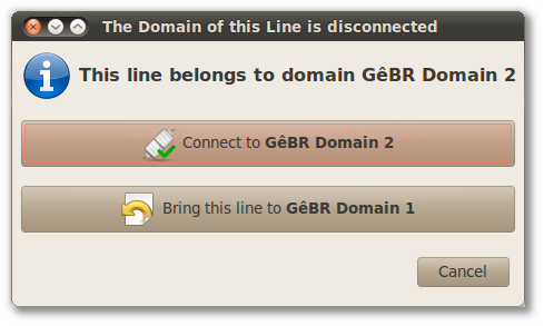
Whenever GêBR is connected to one specific domain, all lines belonging to other domains won't be available for edition. However, a line can be migrated from its original domain to the connected domain. To do so, the line must be selected. In the right-hand side panel, an icon in the upper left corner indicates whether the domain of the line is connected or not. In case the original domain is not connected, by clicking on that icon, GêBR will offer two options:
-
disconnect from current domain and connect to the domain associated to the line; or
-
dissociate the line from its original domain and associate it to connected domain.
Important
Whenever a line is migrated from one domain to another, all data in the BASE directory and in its children will remain in the nodes of the original domain. That is, the data inside BASE path of the line is not automatically migrated.
Figure 3.2. Dialog for lines from domain with disconnected domain
Although GêBR continuously saves all data, sometimes it is desirable to have copies of projects and/or lines in a file (for example, to share them with others or to make backups). To export a project or a line:
-
Select the line or project that that will be saved;
-
Left-click on
 ;
; -
A dialog will be shown. Choose a directory and a name for the file;
-
Left-click on the button to conclude the export.
Tip
GêBR determines the extension automatically, i.e.,
.prjx for projects and
.lnex for lines.
To import projects or lines that were previously exported follow the steps:
-
Click on the button
 ;
; -
Select the desired project or line file to import. Only files with extension
prjzorprjx(for projects), andlnezorlnex(for lines) are allowed; -
Click on the button.
An imported project is added to the list of projects, while an imported line joins the other lines of project that was selected prior to this process. In both cases the imported item is identified with the suffix Imported.
Note
In GêBR, lines may only exist inside a project (see Section 2.1, “Projects, lines and flows”). Therefore to import a line one has to first select an existing project, or create a new one.
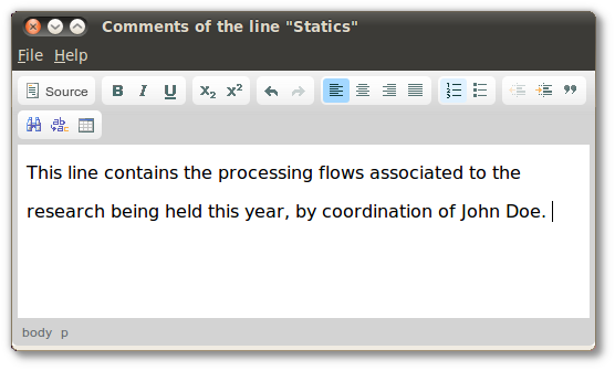
Projects and lines can be commented. The commentaries are free formatted text. While for projects the report is entirely composed only byt the user's commentaries, for lines, the report is created automatically, including not only the user's commentaries, but also information about its flows.
To edit the commentaries of the project or line, follow the steps:
-
Choose a project or line;
-
Click on the button on the toolbar;
-
Choose Edit Comments;
-
Write the commentaries as free formatted text through the built-in text editor;
-
When finished, save and close the editor.
Tip
You can print the report by clicking →
The report can be visualized by clicking on → .
Figure 3.4. View Report
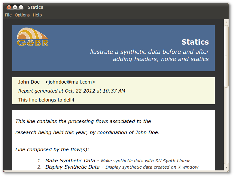
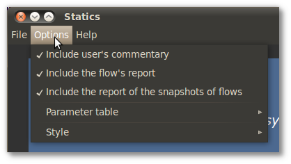
After clicking on View Report, a window will appear showing the report for the project or line. In the case of line's report, some customization options are available:
- →
-
Include comments for this line into the report;
- →
-
Include the reports of all flow of this line;
- →
-
This option will include reports from all snapshots of all the flows that compose this line (see Section 5.4, “Snapshot of a flow”);
- →
-
Allows to choose how much information about the parameters will be shown.
- →
-
Change the presentation style of the report.
Note
The option to include report of flows' snapshots are available on line's and flow's View Report. More information about snapshots can be found on Section 5.4, “Snapshot of a flow”
Table of Contents
In the Flows tab, processing flows are created, edited and submitted for execution. After creating an empty flow, the desired programs can be added to it and the I/O files and parameters can be configured. Once properly configured (GêBR warns if not), the flow can be submitted for execution. Prior to the submission, execution details can be set.
Figure 4.1. Flows tab
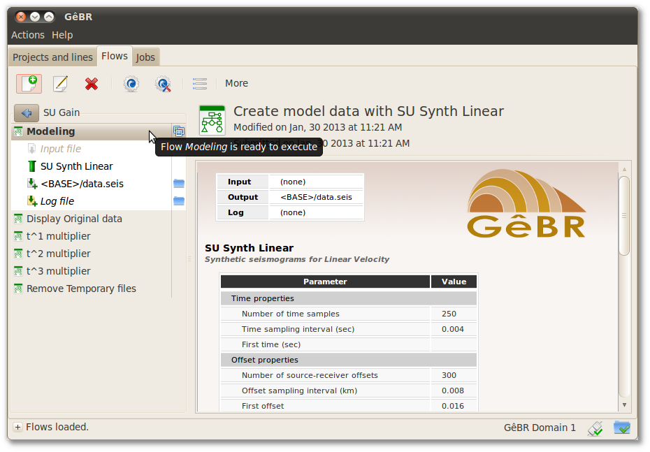
The left panel contains the list of flows of the selected line in the previous tab. The right panel exhibits information of the currently selected flow, divided in two parts:
- On the top basic information such as flow title, last modification date and last execution date can be quickly consulted;
- On the bottom there is a summary of the flow, with the input/output/error files, the programs that compose the flow and the non default parameters. Text searches can be done by pressing Ctrl+F. Additionally, problems in the flow assembly are warned in this window. To go to the summary view, select (single click on) a flow.
In Section 2.2, “Menus, programs and their parameters” a menu was defined as a set of one
or more programs that can process data. These menus are accessible in the
Flows tab, trough the button menu list
![]() presented in the toolbar.
presented in the toolbar.
After clicking the menu list button, a pop-up window is shown with a list of
categories. All menus registered inside GêBR are classified into these categories, which
can be expanded by clicking the  icon on the left.
Note
A menu can appear more than once in the unfiltered list, since it can pertain to any number of categories.
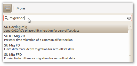
By typing parts of the menu title or description in the text box on the top, it is possible to filter the menus list. This eases the task of finding or discovering a menu when its purpose is known. For example, it is possible to search for menus related to migration (see Figure 4.2, “Filtering the menus list”).
Figure 4.2. Filtering the menus list
In the Flows tab, the button
 creates a flow. Title, description and flow's
author should be provided in the creation, and can be further edited through the button
.
creates a flow. Title, description and flow's
author should be provided in the creation, and can be further edited through the button
.
After following these steps, the flow will appear on the left side of the main window. The right side will show information about the flow.
Tip
It's possible to alter the position of the flow in the list by dragging the flow with the mouse to the desired position.
A processing flow is a sequence of operations defined by the user. These operations, also called programs, are organized into the following categories according to their purpose:
-
Data Compression
-
Editing, Sorting and Manipulation
-
File tools
-
Filtering, Transforms and Attributes
-
Gain, NMO, Stack and Standard Processes
-
Graphics
-
Import/Export
-
Migration and Dip Moveout
-
Multiple Supression
-
Seismic Unix
-
Simulation and Model Building
-
Utilities
After the flow is created, a pop-up appears with the available menus and is possible assemble the flow:
-
Choose one of them and include it in the flow with a double-click.
-
To specify an order to the programs, simply drag and drop the desired programs.
-
Inserted program comes in an enabled state (unless they have required parameters).
-
Some programs have required parameters. To edit or to alter the default parameters, consult Section 4.4, “Editing program's parameters”.
-
To change the program status, right-click over it and choose the first option, Enable/Disable (for more information, see Section 4.3, “Program states”).
Important
To run a flow all the programs listed in the Flow Sequence box must be enabled (
 ).
Otherwise the flow will not be executed as expected.
).
Otherwise the flow will not be executed as expected.
The flow is ready to be executed. Click on
 or on
or on
 to do it (for more information, consult Section 4.7, “Executing flows”).
After the flow has been assembled, it will be visible on the left side of the main window when the Flows tab is selected. The Details box, found on the upper right side of the main window, shows information about the selected flow. The Flow Review box shows a brief of the flow and contains information like input, output and log file, flow's programs and some of its parameters.
Programs can be in two states only, Enabled
()
or Disabled
( ).
If a program is enabled with an error, the icon changes to
).
If a program is enabled with an error, the icon changes to
 .
.
Alternate between these states by using two methods: on the program and then select the desired state from the context menu or using the shortcut Spacebar to change the states of the selected programs. It's possible to select several programs whose state is desired to change by holding Ctrl+ or Shift+.
Tip
Changing a program state does not alter its parameter configuration. This way, alternate between states is an operation completely safe.
Important
Disabled programs
()
will be ignored when the flow runs. This
way, the user can enable and disable parts of
the flow.
Program's parameters compose a set of initial configurations defined by the user.
To edit program's parameters follow the steps below:
-
Select the program from the list and click on
on the toolbar, or just double-click on the
program. The Parameter box will
appear on right side of window over the Flow Review box. -
Edit the program's parameters. Notice that each parameter vary greatly both in size and type. In parameters fields that can be filled with numbers/text, variables can be used (Section 5.2, “Using variables”).
Tip
Click on the button (bottom right corner of the dialog box) to view the program's documentation. This will be certainly useful when the user is editing the programs parameters.
Tip
Click on the button to return to default configurations.
-
All changes are saved automatically, and to close the Parameter box, simply change selection on left side.
In many occasions, it's necessary to extract data from an input file and/or generate as a result an output file, or even an log file in case an error occurs.
To associate an input, output and error file to a flow, follow these steps:
Figure 4.3. Input file setting
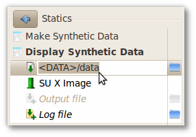
-
Select a flow, in the Flows tab.
-
Below the selected flow, the programs and entries with input, output and log files will be shown. To edit files paths, just double clicking on them.
-
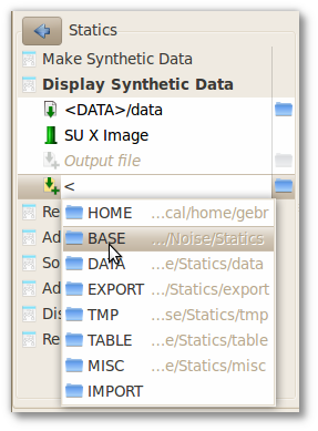
Type in the path (important folders can be consulted/choosen by typing <) or click on
 to browse for the file (see
Section 8.2, “Accessing remote files”).
to browse for the file (see
Section 8.2, “Accessing remote files”).
For using the folders associated to the line, choose them like above or use the feature of autocomplete of the important folders of this line. For more information, see Section 3.3, “Important folders of a line”.
Figure 4.4. Autocomplete of paths
When a path is chosen for the
flow's input/output, their file
paths will appear in entries, indicated by the icons
 and
and
 ,
below and above the flow's programs (if there are
any).
,
below and above the flow's programs (if there are
any).
Note
If necessary removing a set from the list, select them by pressing right-click and then click on .
The clipboard provides the popular set of tools known as copy and paste. A flow (or set of flows) can be copied to the clipboard and paste back to the same line or to other lines. In the same manner, a program (or set of programs) can be copied to the clipboard too, and can be paste to the same flow or to other flows.
To copy flows or programs to the clipboard, first
select them with the mouse, and then use the button
 or press the usual shortcut
Ctrl+C. After copying the user can paste it
by clicking on the button
or press the usual shortcut
Ctrl+C. After copying the user can paste it
by clicking on the button
 or by simply using the shortcut
Ctrl+V.
or by simply using the shortcut
Ctrl+V.
To delete a flow (or set of flows) and a program (or set a programs),
select them then click on
.
It's possible to handle several flows at once by pressing Ctrl+ or Shift+.
Caution
GêBR does not ask for confirmation before deleting programs from a flow.
Caution
Deleting a flow implies that all snapshots of the flow will be equally deleted (see Section 5.4, “Snapshot of a flow”).
Once assembled, a flow can be executed in two ways:
-
Run - Basic execution (
).
-
Setup and Run - Advanced execution (
).
More than one flow can be submitted for execution at once. To make a multiple selection, click over the flows, while Ctrl is pressed or use the arrow keys while Shift is pressed.
After being triggered, the execution can be followed in the same window or, for more detailed information, in the Jobs tab (see Section 4.8, “Following the execution of a flow” and Chapter 6, The Jobs tab).
By clicking on , the flow will be immediately
submitted with following default settings:
- In case of multiple flows, the default is to execute them sequencially (one after another).
- The execution starts immediately.
- Some flows give rise to jobs, that can be splitted in smaller parts, called tasks. In this case, these tasks are distributed among available processing nodes, according their nominal capacity (total number of cores). If the job cannot be splitted it will be sent to the best available processing node at time. (For more information, see Section 8.3, “Parallelized processing”.)
- The job execution will compete for resources with other processes. (For more information, see Section 8.4, “Priority of execution”).
This is the fastest way to execute, skipping the configurations of the Run and Setup. Useful keybinds are available here: Ctrl+R runs the selected flows one after another; Ctrl+Shift+R runs the selected flows parallely (keybind activated just if multiple flows are selected).
Note
Some execution configuration (like group's nodes, number of tasks splitted and priority) can be saved using Setup and Run. That configuration is going to be a new default for basic Run. (For more information, see Section 4.7.2, “Setup and run”.)
Many execution details can be set before triggering a job. After setting, click on Run to execute the job.
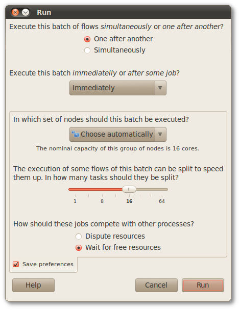
By clicking the button , the following options can be tunned:
- When will the jobs be executed? This option just
appear if multiple jobs are selected for running (multiple
execution).
- One after another: Jobs are executed one after another, according the order of the flows in the flows' list. Each job is triggered only when the previous job has been concluded.
- Simultaneously: All jobs are dispatched simultaneously. Note that this option is not feasible if there is dependency between flows.
- The beginning of the execution process can be delayed to wait the conclusion of some running job or it can be triggered immediately (default).
- Where should the jobs be dispatched? Nodes or set of nodes can be specifically choosen to process the jobs. A special option is Choose automatically. It instructs the maestro to submit each job for the node or set of nodes less overloaded of the domain.
- The number of tasks settled to split the jobs. This parameter is valid only when there is a parallelizable job among the selected jobs. The nominal capacity is given by the number of cores of the group of nodes that are in charge of the execution of the jobs. For non-parallelizable jobs, this parameter is automatically set to 1. For more information, consult Section 8.3, “Parallelized processing”.
- How does the job compete for resources with other processes of the system? Choosing Dispute resources, each job will be dispatched with default priority. Hence, they will compete equally for system resources with all other running processes. This could overload a processing node with too many running processes. By the other hand, choosing Wait for free resources, the execution of each job will delayed whenever the processing node has other process to operate on. This is particularly interesting we running jobs on desktop machines. In that scenario the user experience will not be degradated by the job execution. For more information, consult Section 8.4, “Priority of execution”.
Note
Decisions made about itens 3, 4 and 5 above can be saved for future executions by checking Save preferences.
Example 4.1. Parallel execution
On a multi-core system, create a flow according to the following steps:
- Insert a loop with thirty steps (see Section 5.3, “Flows with loops” for further details about loop).
- Insert a sleep program with parameter set of one second.
- Open the Execution detailed window, and set the minimum number of cores (one core) to execute the flow and Press run.
- Execute step three again, but now with the maximum number of cores (nominal capacity).
It can be seen that:
- For the minimum number of cores, the flow lasts thirty seconds to be executed. That is because the only core is responsible for the thirty sleeps step.
- For the maximum number of cores, the flow is executed much faster. For more than thirty cores, it lasts only one second. On a thirty cores system, each sleep is executed by one core, so that a fast distributed execution is possible.
This flow is parallelizable only because one step of the loop is totally independent of another, so, in a system with multiple machines and multiple cores, this flow can be divided to execute all their tasks on the same time, making the execution faster. Therefore, all flows with the same characteristic can take advantage of it.
Flows submitted for execution generate jobs (see Section 2.3, “GêBR players”). The status and output of the yielded job can be followed in the same window, still in the Flows tab. A bar in the botton of the window will appear to keep the history of the last jobs dispatched for execution. Through buttons in that bar it is possible to switch among the results of the many jobs.
Each job execution is represented in the bar as a button, composed by:
- an icon representing the status of the execution, and
- an integer number, which is associated to the number of executions of that flow.
Differently from the Jobs tab, in the Flows tab it is presented just a quick view of the job. However, the arrow button takes the view to the Jobs tab, where full information about the job is available.
When multiple flows are dispatched for execution, instead of staying in the same window, GêBR automatically switches to the Jobs tab, where all the executions can be seen together.
Table of Contents
Although GêBR continuously saves all modifications made to flows as well as to projects and lines, sometimes it is useful to dump flows to file. This can be used to share flows among users, for instance, or to generate backups.
Import and Export actions are accessible through the → and → on toolbar.
To export flows, select as many flows as you want with help of the mouse and keys
Ctrl (for single selection) or Shift (for multiple selection), then
activate the export option at menu. A dialog box
Save flow will pop up, allowing the user to browse for the target directory and
chose the filename (GêBR will automatically determine the extension flwx).
In case of importing flows from a file, the imported flows will be listed along with the other flows of the active line, at the bottom of the list and with the suffix (Imported) added.
It is usual in the course of processing data that many flows may depend on some fundamental quantities, like acquisition parameters, for example. Those quantities may be provided explicitly to each flow. Consider however a scenario where one or some of those quantities have to be redefined. The user would have to go through all flows which depend on them making the necessary updates. Despite possible, this procedure is error-prone and time consuming. A better approach would be centralize the definition of those common quantities, in such a way that a change on them would be automatically propagated to all flows where they are employed. This central place for definition of these quantities is the Dictionary of variables.
Variables are ways to hold numbers or text strings. Numerical variables are defined by arithmetic expressions involving constants and/or other numerical variables. Text string variables are defined by concatenating constant text strings with other numerical or text string variables.
Variables may be used to define programs' parameters directly or by means of inline expressions, i.e. expressions written directly on the parameter's entry box.
The Dictionary of variables is to interface to handle all the
variables. It is accessed through the icon  , in the
menu of toolbars of the Projects and
Lines and Flows tabs.
, in the
menu of toolbars of the Projects and
Lines and Flows tabs.
GêBR has three levels of organization (see Section 2.1, “Projects, lines and flows”). The variables, thus, have three levels of visibility:
- Project's variables are visible to all flows associated to lines of the project;
- Line's variables are visible to all its flows;
- Flow's variables are just visible to the flow itself.
Figure 5.1. Dictionary of variables
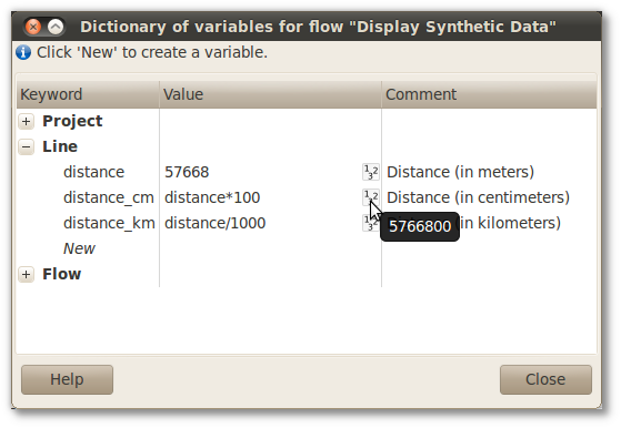
The dictionary validates the variables dynamically, revalidating and recalculating them as soon as anything is changed in dictionary. Programs with errors are automatically revalidated too (see Section 4.3, “Program states”).
Positioning the pointer over the icon of the variable's type, the user can check the solved
expression and see the actual value of the variable. If the Dictionary of
variables finds an error among the variables, it is going to exhibit the icon
 and an explanation of the error. Reordering the
variables of the dictionary can be done by drag and drop. Since a variable can just use another
variable above it, this feature turns the declaration of variables more flexible and
dynamic.
and an explanation of the error. Reordering the
variables of the dictionary can be done by drag and drop. Since a variable can just use another
variable above it, this feature turns the declaration of variables more flexible and
dynamic.
Besides variables and expressions, some predefined functions can be used:
Table 5.1. Available functions
| Function | Sintax |
|---|---|
| Square root | sqrt (value) |
| Sine | s (value) |
| Cosine | c (value) |
| Arctangent | a (value) |
| Natural logarithm | l (value) |
| Exponential | e (value) |
| Bessel | j (order, value) |
The character [ (open bracket) is used to see all the available variables for auto-completion while writing an expression.
Navigate over the fields can be done by using the keys Enter, Tab or with the .
Tip
To use the variables in text entries, the variable name need to be embraced by square brackets: [ name-of-the-variable ].
To insert a literal square bracket in a text entry, double it, that is, [[ yields is a literal [.
Example 5.1. Using the dictionary
Dictionary is a very useful feature for using a same value multiple times. It is also useful for naming variables, making a flow's parameters more intuitive. For example:
- Import a demo named Making Data.
- Check the line named Shot Gathers.
- Open the Dictionary of variables, on Flows tab.
It can be seen that:
- Some of the variables are line's variables (width, height...). Changing width and weight, all images generated by X Image (on this line) will be changed according to the new value set. Instead of setting each new value, all values can be changed at once.
- Still on Shot Gathers, select the flow Single Shot Sixty Degrees. By checking Dictionary of variables, it's seen that there are some variables related to this flow and these variables are only used on this flow. Also, there are some variables used twice (like dz). It's important to check that the names of each variable represent a meaning on its context : d (z or x) are related to sampling interval; f (z or x) are related to first sample.
The notion of a loop refers to a series of commands that continues to repeat over and over again, possibly changing a little, until a condition is met. For example, suppose the user needs to extract many common-offset sections of a data. Instead of writing a flow to extract each common-offset section individually, or refurbish a base flow, changing manually its target offset, a loop over the offset could be used to sequentially extract all common-offset sections.
The Loop is a special menu from the category Loops that has a totally different usage compared to the remaining menus of GêBR. Here these differences are presented.
Whenever the Loop is added, it appears on the top of the flow. That happens to indicate that the flow is going to be executed more than once, according to the parameters set for loop. (see Section 4.4, “Editing program's parameters” for further details).
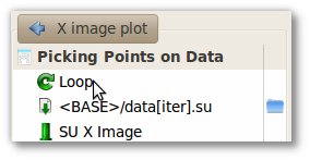
After the Loop is added, a new variable, the iter, is available (see Section 5.2, “Using variables”). The value of this special variable is modified on each iteration (increasing or decreasing), according to the parameters set.
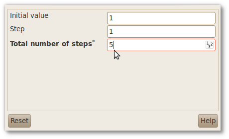
Figure 5.3. Loop parameters
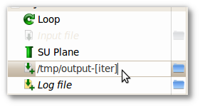
For instance, the output of each step of the Loop can be defined to a file with a name identified by the step, output-<number-of-steps> (see Figure 5.4, “Usage of iter variable”).
Figure 5.4. Usage of iter variable
Tune all program's parameters of a flow can be time consuming. Usually the best setup of parameters is only found by trial and error. It could be distressful have to change a good flow's setup to try a different one, in aim of found something better. To alleviate this stress, GêBR offers the snapshot feature. A snapshot is a record of the complete flow's state at the time, including all programs that build the flow, all program parameter values, the state of the dictionary of variables, and input and output files. After take a snapshot, the user can change anything in the flow's setup without the fear to corrupt the flow, because it is always possible to revert the flow to the state it was when the snapshot was taken.
Snapshot can also be used to keep equally important different states of a flow. For instance, consider a flow to extract a common-offset sections from a data set. One valuable setup is the one that extract the common-offset section for the smallest offset, while other important setup is the one to extract the common-offset section for the biggest offset. Both states can be saved by means of snapshots. Furthermore, both snapshots can be executed at once.
An alternative to snapshots would be is to save many different flows, one for each version, but with the drawback of having a crowded flow's list.
To take snapshots of a flow, on the toolbar of Flows tab, use the option → or press Ctrl+S. A dialog box will appear requesting an one-sentence description of the snapshot. That description is further used to identify it as long as the timestamp of the snapshot.
To see the saved snapshots, just left-click on
 by the title of the flow in the flow's list.
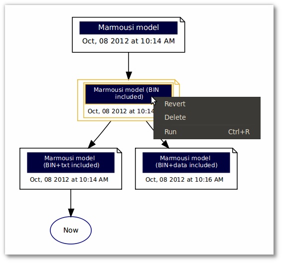
The graph below indicates from which version each snapshot was derived from. The start of arrow indicates the origin and the end indicates the derived version. The special mark Now highlights from which snapshot the actual state of the flow derives.
Figure 5.5. Snapshots on GêBR
In this view, it is possible select as many snapshots as necessary by just clicking over each snapshots. To deselect a snapshot click again over it. To clear the entire selection click on the white area in this view.
Any action taken will affect all selected snapshots. Possible actions are Revert, Delete and Run.
-
Revert
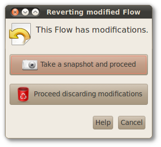
Revert means that the flow will be restored to how it was at the moment the snapshot was taken. If the actual state of flow is unsaved by means of a snapshot, prior the revert action the user is inquired about taking a snapshot of the actual state of the flow or discarding this unsaved state and then proceed.
-
Delete
Delete a snapshot is a permanent action, that cannot be undone. Whenever a snapshot is deleted its descendents are linked to the predecessor of the deleted snapshot to keep the idea of ascendence.
The Delete key can be used instead the context menu option.
-
Run
Running a snapshot is like running a flow (see Section 4.7, “Executing flows”). The advantage of doing this is the possibility of executing a snapshot without having to revert to it. Thus, saved flows can be tested without changing the current one. As with flows, Ctrl+R runs the selected snapshots one after another; Ctrl+Shift+R runs the selected snapshots parallely (keybind activated just if multiple snapshots are selected).
Example 5.2. Using snapshots
Take the program SU Plane for that example. That program create common offset with up to 3 planes, and there are two possible output options for that flow: image plot, using program X Image or postscript image, using PS Image.
To solve this issue (two possible outputs for a flow) without the need to create two separate flows with small differences, it is possible to take two snapshots: one for image plot, and the other for postscript.
To do that, following the steps below:
- Assemble the flow with two programs, SU Plane and X Image.
- Takes a snapshot of this flow, with some description like "Common offset with image plot".
- Remove the program X Image of the original flow, and add a program PS Image, with some output file like "plot.ps".
- Takes a snapshot of this new flow, with description like "Common offset with postscript image".
Now, with only one flow can run two different plots for the data generated from SU Plane.
The option → allows the user to add comments about the selected flow, just like the option presented in the Projects and Lines tab. Analogously, the option → allows the user to visualize the report of the current flow. The difference is that the line's report can include the flow's report. Consult Section 3.6, “Report of a project or a line”.
Table of Contents
The jobs submitted for execution in the Flows tab can be followed in Job Control tab. As anywhere else in GêBR, the information presented here is preserved even when GêBR is closed. It is possible to consult the flow's state (if it has ended, has failed or is queued), the results and the submission details.
Figure 6.1. Jobs tab
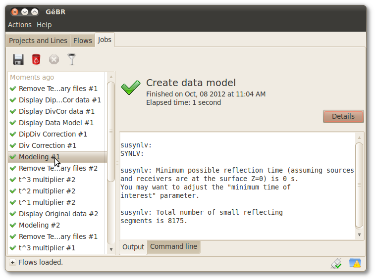
As seen in Section 4.7, “Executing flows”, GêBR switches to the Jobs tab whenever multiple flows are executed, in other cases, the user can switch through Flows tab, using a arrow on info bar to fast view of jobs, localized on bottom of tab.
This tab has three sections:
Toolbar: Operations over jobs
Left Panel: List of jobs
Righ Panel: Details of a selected job
In this tab the user can follow and, if so desired, interrupt the flow's execution. The available commands are:
-
Save (
 ) to disk the output of the selected flow up to the moment.
 -
Clear job (
 ).
Eliminate from the Jobs the selected job. Caution is needed because the
process is irreversible.
).
Eliminate from the Jobs the selected job. Caution is needed because the
process is irreversible.The user can only clear jobs that are not being executed (
 or
or
 ).
). -
Cancel this job (
 ). The user can cancel a running (
 )
or queued (
)
or queued (
 ) job.
When a job is terminated in this manner, the job will be marked
with
.
) job.
When a job is terminated in this manner, the job will be marked
with
.
-
Filter jobs (
 ). The user has the option to see just the desired
results.
). The user has the option to see just the desired
results.
Tip
As in anywhere else in GêBR, many of the toolbar functionalities can be accessed through the context menu, using the mouse's right button.
In the left panel, GêBR presents a list of flows executed by the user, ordered by moment of execution. Each exhibited flow can be in one of four states:
-
Running (
): job in execution;
-
Finished (
): already completed job;
-
Canceled (
): stopped
- Queued (
): waiting for another job.
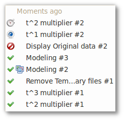
Beside the job name, an icon (
) appears to represent that this job came
from an execution of snapshot (see Section 5.4.2, “Snapshot actions”).
In the upper part, information of the selected flow is exhibited. More informations are shown clicking on Details. Among the exhibited information there are:
Description of related flow. If the job is from a snapshot, the icon
is displayed along with the description of snapshot.Moment of start/finish of the flow.
Elapsed time in execution
Input/output files
The nodes group in which the flow were executed
Which machines were effectively used in
the group and how the distribution of the work was done can be
consulted by clicking on
 .
.
Figure 6.3. Details of job execution
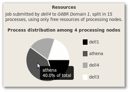
The provided information are:
-
Maestro
-
Domain
-
GêBR (client)
-
Total number of processors used in the execution
-
Distribution of the jobs to the nodes
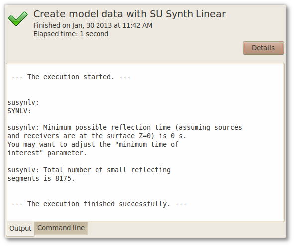
The results (standard output) of the flow are shown. The redirected output are not exhibited. Right-clicking on this window, an Options menu is exhibited, by which the user can enable the automatic word wrap and the automatic scroll of window as the output is being shown.
The user can also consult the command lines executed by GêBR. He just needs to visit the Command Line tab. The command lines are portable and can be copy-pasted to execution on a terminal.
Table of Contents
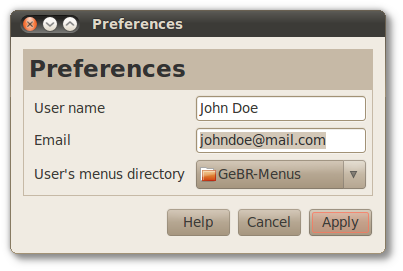
From the menu, the user can access the and configure the settings. If the user's enthusiasm for GêBR has lead to read the whole manual, then the user has probably used almost all available features found in these options. But just in case, the user will find the documentation for these options below.
The details the user provides in the dialog box will be adopted as the default by GêBR. Specifically:
-
User name: will be used as the default for Author, when the user creates projects, lines and flows.
-
Email: will be used as the default for Email, when the user creates projects, lines and flows.
-
User's menus directory: will be the default directory where GêBR's Menus are maintained (
mnufiles).
Figure 7.1. Global GêBR preferences dialog box
This option helps the user to configure all the necessary connections to work properly GêBR.
The connection assistant explains how to connect to a maestro, its servers and enable remote browsing into a domain (for more information, see Section 7.3, “Maestro/Nodes configuration” and Section 8.2, “Accessing remote files”).
The Maestro/Nodes Interface has three parts:
-
Maestro: central unit of coordination of multiple machines (for more information, see Section 2.3, “GêBR players”).
-
Nodes: choose the nodes associated to the current maestro.
-
Groups: configure the groups of nodes on the current maestro.
Figure 7.2. Maestro / Nodes configuration dialog box
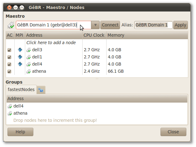
In the upper part of the Maestro/Nodes Interface (see Figure 7.2, “Maestro / Nodes configuration dialog box”), there is an entry in which the user can put the desired machine to use as maestro. A requirement is that the maestro must be installed on that machine. The state of the connection between GêBR and the maestro is shown by the right-side icon:
connected (
 )
)disconnected (
 )
)error (
)
Once the maestro has been selected and the connection has been successfully established, the user can associate nodes to domain conducted by that maestro.
Each line of the nodes window represents each machine into maestro's domain. The lines have some columns:
To add a new machine, click over New and enter the hostname or IP address of the machine.
It's possible to employ a subset of the machines into the maestro's domain. This can be done through the creation of groups of machines.
The administration of the groups is in the bottom part of the Maestro/Nodes interface (see Figure 7.2, “Maestro / Nodes configuration dialog box”).
To create a group, click over a node
in the list and drag it to the
 icon.
A text box will be prompted for the name of the group. Groups
with same names are not allowed.
icon.
A text box will be prompted for the name of the group. Groups
with same names are not allowed.
Example 7.1. Using the groups
Using groups is very useful when it's necessary to run a flow in a subset of machines different from the default (For more information, see Section 4.7.2, “Setup and run” ). That's useful, Because sometimes it's desired save resources from some processing nodes to not overload all of them.
For example:
- Choose a subset of processing nodes
- Create a group with them.
- Give a name for the group.
- Create a parallelizable flow (see Section 8.3, “Parallelized processing” ).
- Open the Execution settings window on Flows tab (see Section 4.7.2, “Setup and run” ).
- Set the maximum number of cores (nominal capacity) to execute the flow.
- Set the group node desired.
- Press run.
- Go to Jobs tab.
- Click on Details.
- See the nodes group in which the flow was executed (see Section 6.3, “Right panel” ).
It's easy to see that the execution was distributed in the nodes of subset (group) chosen by the user and not in all the processing nodes.
In → menu, there are samples to be imported.
GêBR offers bundled samples for download in its hostpage, hostpage like gebr-menus-su package. Here are some samples this package provides:
- Dip Moveout : Ilustrates different types of DMO processing
- Velocity Analysis : Illustrate some velocity analysis processes
- NMO : Illustrate normal moveout corrections and stacking
- Ray Tracing : Illustrates different ray tracing programs
- Migration Inversion : Illustrates different processes of migration inversion
- Time Frequency Analysis : Illustrates chirpy data in the time-frequency domain
- Deconvolution : Illustrate a random noise attenuation via F-X deconvolution
- Filtering : Ilustrates different filtering processes
- Trace Headers and Values : Illustrates several applications to the trace headers and values of keywords
- Plotting : Illustrates different plotting programs
- Velocity Profiles : Illustrate several types of velocity profiles
- Muting : Illustrating a picking in a data, and your result after applied mute
- Synthetic : Show several demonstrations about synthetic data creation
- Amplitude Correction : Illustrates the amplitude correction on synthetic seismic data
- Offset Continuation : Ilustrates the use of Offset Continuation method
- Block : Creates a data set of the form required by the "block" program.
- Stacking Traces : Illustrating the usage phase weighted and diversity stacking
- Vibroseis Sweeps : Illustrates using SUVIBRO
- Making Data : Illustrating the construction of common offsets and shot gathers
Once imported, the associated flows can be readily consulted or executed (consult Section 4.7, “Executing flows”).
Table of Contents
GêBR can take benefit of the resources of multiple processing nodes. To handle it, GêBR is segmented in three layers:
Note
GêBR can be connected to only one domain at once. The domain, in turn, can be composed by many processing nodes. However, to be part of the same domain, those processing nodes must share the file system containing the user's home directory. This is usually provided by Network File System (NFS) infrastructure.
GêBR model comprises communications between processing nodes (see Figure 2.2, “Communication layout between GêBR players”), namely:
- Between client and maestro (the domain representative).
- Between maestro and other nodes.
All connections are performed using Secure Shell (SSH) protocol. SSH is intended to provide secure encrypted communication over a network. A login password may be asked multiple times to establish such connections. This can be cumbersome, if there are a lot of nodes under the maestro domain.
The SSH public-key authentication is an alternative method to establish connections which eliminates the need of requests for passwords. Despite less annoying, this method is equally secure. It is based on public-key cryptography, where encryption and decryption use public/private key pair for authentication purposes. The maestro knows the public key and only the client knows the associated private key.
By checking the option Use encryption key to automatically authenticate the next session on password dialog, GêBR will use public/private key authentication. Once this operation is successfully done, there will be no need to type the password to connect to that maestro through GêBR. Analogous behavior occurs in the connection between maestros and nodes.
Figure 8.1. GêBR public-key authentication
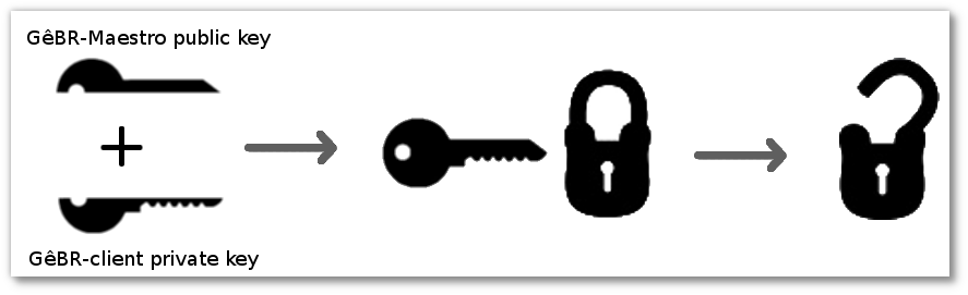
Alternatively, the private/public key pair can be created without GêBR (consult here for more information).
GêBR infrastructure comprises GêBR, maestro and nodes as main actors (see Section 8.1, “Intercommunication between players”) and the processing files, therefore, may be on different places than the user's node.
No matter the node where the file is, it can be accessed through the remote navigation (see window below).
In two places GêBR will not browsing the nodes filesystem: Import/Export of projects, lines or flows. On these cases, backup can be saved on the local machine, instead of remote nodes.
Figure 8.2. Remote browsing of files
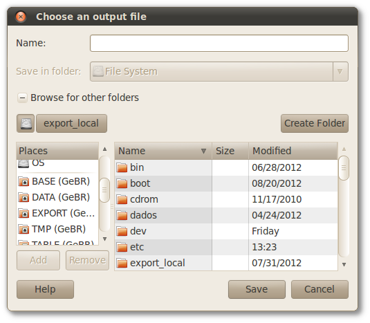
GêBR puts markers (bookmarks) to the important folders of the line in context (see Section 3.3, “Important folders of a line”). They aim to facilitate the access to the files of the line.
Note
In external file browser (say Nautilus), these bookmarks will appear there too. They disappear when GêBR is closed.
GêBR takes advantage of the multi-core feature of most of the recent machines. The execution of repetitive flows can be optimized by this resource. If the flow has Loops and is parallelizable (given some criteria, shown below), the execution performance based on the number of processors can be adjusted.
GêBR also takes advantage of the number of processing nodes connected to the user's maestro. The resources of every node can be effectively employed to improve the performance.
Accordingly, GêBR can parallelize the flow if:
- the processing node has a multi-core architecture or;
- the maestro is connected to multiple nodes.
and if the flow is parallelizable.
To be considered parallelizable, besides having a loop, a flow must achieve one, and just one, of these criteria:
- The flow does not have an output file;
- The flow has an output file which depends on the iter variable (see Section 5.3, “Flows with loops”);
- The output of each step of the loop is not the input of any other step of the loop.
- Flows with MPI programs (see section Section 8.5, “Support to MPI programs”).
The level of parallelism of a job execution can be adjusted by the Advanced Execution settings (see Section 4.7.2, “Setup and run”).
In case the flow is not parallelizable (i.e., does not fit any of the above conditions), GêBR runs the job in the choosen node.
Computers, nowadays, are multitasked, what means that multiple things can be done at the same time. When many tasks are executed at the same time, the computer can get overloaded and decrease its performance. Seismic processing, particularly, can exhaust the computer resources.
GêBR has a feature that overcomes the issue of overloading due to multitasking, by enabling the execution of the flows in a Wait for free resources state:
Two options are available (see Section 4.7.2, “Setup and run”):
-
Dispute resources (the execution of the flow is going to dispute for the computer resources with all the other active programs).
-
Wait for free resources (the flow is going to wait its turn to execute and try not to overload the system).
Technically, when running in Wait for free resources mode, GêBR will reduce the execution priority of the task, meaning it will tell the computer that "it can wait more important things to be done". This is the case when the user has other things to do while waits the calculations to be done.
The Share available resources mode means GêBR will use greater run priority for the task, and that implies it will act as a foreground process, demanding more resources. It's the "I need this done now" mode, when the user needs the job to be finished as soon as possible, and doesn't care if it will fight for resources with other programs.
If GêBR is the only program executing on the node, i.e., it doesn't have a challenger for the computer resources, then both states corresponds to the same situation. This is the "nightly job" situation, when (theoretically) no one is using the processing nodes and some jobs are left to be done for the next morning.
Some programs, known as parallel programs, deal themselves with the distribution of their computations among many nodes. In this way, those programs are much more efficient, exploit all available resources to run faster. Technically, they employ a infrastructure known as MPI. GêBR supports parallel programs.
There are many implementations (flavors) of MPI, but the most widely used are OpenMPI and MPICH2. OpenMPI is an open source implementation and has influence of three earlier approaches: FT-MPI, LA-MPI and LAM/MPI. The MPICH2 is another widely used implementation and is based on the MPI-2.2 standard.
GêBR supports both OpenMPI and MPICH2. However, MPI programs can only run on nodes that support the execution of MPI. Thus, for GêBR support of MPI, the user must have acces to nodes/clusters that also support it.
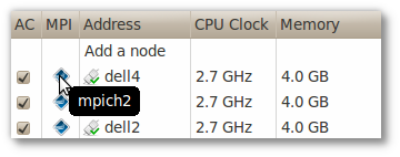
In the maestro/nodes interface, in the MPI column, an icon indicates whether the node supports MPI. Roll over the icon to check the flavors of MPI available on that processing nodes. The parallel program can be executed just on processing nodes that support the same flavor as the one used in it.
Figure 8.3. Indication of MPI availability
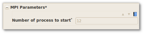
To run an MPI program, first it's necessary create a menu in DêBR and choose the proper MPI implementation to the program. Then import it in GêBR. With double-click over the MPI program in the Flows tab, the number of processes to be used by that MPI call can be seen.
Figure 8.4. MPI settings
The system administrator can configure global options appliable to everyone that starts GêBR for the first time.
GêBR verifies the existence of an environment variable
(GEBR_DEFAULT_MAESTRO) to suggest a maestro.
The syntax of
this variable is maestro_A, description_A; maestro_B,
description_B.
For instance, if the administrator sets GEBR_DEFAULT_MAESTRO as
127.0.0.1, My first maestro; 100.00.00.0, My second maestro;
then, on the first time or through Connection Assistant
(see Section 7.2, “Connection assistant”),
GêBR will offer the following options:
- 127.0.0.1 as the default maestro with description 'My first maestro'
- 100.0.0.0 as another available maestro with description 'My second maestro'
Additionally, GêBR can also automatically
add processing nodes. This
configuration can be done through a file in the path
/etc/gebr/servers.conf.
The syntax of this file must be the names of the nodes enclosed by brackets.
For instance, if the administrator sets /etc/gebr/servers.conf
with
				[node1]
				[node2]
				[node3]
then for every user with that maestro, the processing nodes node1, node2 and node3 will be available.
D
- DATA, Important folders of a line
- Dictionary of variables, Using variables
- Domain, GêBR players, Important folders of a line, Changing the domain of a line, Setup and run, Connection assistant, Maestro
E
- EXPORT, Important folders of a line
G
- GêBR
- the interface, What is GêBR?, GêBR players, Intercommunication between players
- GêBR Project, GêBR Project
H
J
- Job, GêBR players
L
- Line, Projects, lines and flows
- Loop, Flows with loops
M
N
P
- Parameters
- supported types of, Menus, programs and their parameters
- Processing flow, Projects, lines and flows
- Processing node (see Node)
- Processing nodes, Important folders of a line
- group of, Groups
- Program, Menus, programs and their parameters, Creating flows
- parallel, Support to MPI programs
- Project, Projects, lines and flows
R
- Remote browsing, Important folders of a line
- Report
- of a flow, Report
- of a line, Report of a project or a line
- of a project, Report of a project or a line
S
- Snapshot
- actions, Snapshot actions
- of a flow, Snapshot of a flow
- taking snapshot, Taking snapshots
T
- TABLE, Important folders of a line
- Task, Run
- TMP, Important folders of a line
V
- Variable, Variables
D
- Dictionary of variables
Place where the variables are defined.
See Also Variable.
- Domain
Set of processing nodes, sharing the same file system, which can cooperate to run processing flows.
See Also Maestro, Processing node.
G
- Group
Subset of processing nodes of a domain.
See Also Domain, Processing node.
M
- Maestro
A processing node in charge of intermediating the communication between the GêBR interface and the processing nodes of a domain.
See Also Domain, Processing node.
- Menu
Representation of a single program or a set of programs.
P
T
- Task
Piece of job to be done.
See Also Job.
V
- Variable
Value or information stored for posterior use.
See Also Dictionary of variables.